ASPRO2 User Manual

Revisions :

• ASPRO 2 software version 0.7 (February 2011) : added Target editor / calibrator support / interoperability with LITpro and SearchCal
• ASPRO 2 software version 0.6 (September 2010) : added OIFits support
• ASPRO 2 software version 0.5 (June 2010).

Table of contents

Description

This document will give general information on the new version of ASPRO named "ASPRO 2" to constitute the "ASPRO2 User Manual".

ASPRO 2 is a Java standalone program that helps you to prepare observations on various optical interferometers.

Supported interferometers and instruments

• VLTI (Period 84 - 87)
  • MIDI (2T)
  • AMBER (3T)
  • PIONIER (4T starting from P86)
• CHARA
  • CLASSIC (2T)
  • PAVO (2T, 3T)
  • CLIMB (3T)
  • VEGA (2T, 3T, 4T)
  • MIRC (4T)

Several xml configuration files are provided in the ASPRO 2 software package and will evolve in future releases.

Please give us your feedback if you want other interferometers or instruments to be supported or if you find mistakes in the configuration :
we are trying to maintain the configuration as exact as possible but it is really difficult to have the correct information about instruments ...

Main functionalities

• Dynamic User Interface : any change made on widgets is taken into account on plots immediately
• Load / Save an observation file : allows the user to save his work at any moment. The xml file produced can be reopened later (for off-line use, for example), and is convenient to save all information relative to a list of targets, which can be sent to collaborators, observers at the interferometer, etc...
• Observability plot : represents time intervals when the source can be observed with transit and elevation marks : night and twilight zones, delay line compensation for the selected base lines, (best) PoPs (CHARA), telescope shadowing (VLTI) and zenithal restriction
• UV Coverage plot : shows the projected base lines on the UV plan and an image of the source model to see the UV coverage of the source
• Interferometer sketch to display the selected base lines
• Target editor : show complete target information, edit missing target magnitudes and associate calibrators to your science targets
• Model editor : each source can have its own object model composed of several elementary models (punct, disk, ring, gaussian, limb darkened disk ...)
• Interoperability using SAMP (VO protocol) :
  • LITpro to prepare your model fitting using the generated OIFits file and the object model of the current target
  • SearchCal to search calibrators for the science target
• Observing Blocks can be generated :
  • for VLTI instruments (MIDI, AMBER and PIONIER) to be imported in the ESO P2PP software
  • for CHARA VEGA instrument using the Star list format
• OIFits file generation with error and noise modelling
• Export (/Print) : every plot can be exported as either a PNG image or a PDF document. Of course the PDF output is better as it uses vector based graphics and any PDF reader can print it correctly (no "Print" button yet, please print the PDF output using your favorite pdf viewer !)
• Standard JMMC actions : feedback report, news, release notes and FAQ

Future functionalities

• Multi configuration support to have an overview of the UV coverage of the source observed with different configurations
• OIFits explorer (visibility plot)
• User-defined Models
• ...

Requirements

• Java Runtime Environment (JRE) 1.5 or better (Sun JRE 1.6 is recommended as it incorporates Java Web Start) : see Java information
• any PDF reader to display and print any exported plot
• Internet connection to resolve star identifiers using the CDS SimBad service

How to get and run ASPRO 2 ?

An internet connection is required to use the Java Web Start and run the latest release : ASPRO 2.

Once downloaded, you should have a shortcut icon "Aspro 2" on your desktop (mac and windows only) :

Alternatively you can start it again later using the Java Web Start Viewer and click on "Aspro 2" :

javaws -viewer

If Java Web Start is not working properly on your environment, you can download the Aspro 2 Jar and run ASPRO 2 using the following command :

java -Xms128m -Xmx256m -jar Aspro2.jar

Look at the JMMC application page to see the complete list of JMMC applications including both ASPRO and ASPRO 2 software packages with related links to news, release notes and FAQs...

Note

you can run multiple instances of ASPRO 2 at the same time, but it may be confusing when you want to interact with SearchCal

Guided tour

How to run a simple preparation scenario ?

1. Launch ASPRO 2
2. Set the main observation settings (interferometer, instrument, configuration ...) and constraints (date ...)
3. Enter your observation targets using the the SimBad star resolver
4. Navigate among tab panels to see outputs and other options

To complete your observation preparation, you can :

• use the Target Editor to define your object models and your calibrators manually
• or use SearchCal to find calibrators automatically
• export to PDF documents, Observing Block or OIFits files ...

Of course you can save your complete observation setup using File menu / Save action to use it later ...

Notes

On every plot panel, you can use the PDF button or the File menu / Export plot to PDF action to export it as a PDF document (and print it).
Alternatively you can export the plot as a PNG image by using the plot context menu (right mouse click) and choose the Save As action.

Plots are zoomable using the mouse wheel or making a mouse drag: left to right to zoom in, right to left to reset the zoom.

Main observation settings

The main panel is always present at the top of the application window to let you change main settings :

• Selected Interferometer + the ESO observation period (VLTI)
• Selected Instrument among available instruments for the selected interferometer (and period)
• Selected Base line Configuration. Note: this list contains only available base lines for the selected instrument and period (VLTI)
• Pipes Of Pan (PoPs) configuration (CHARA) : this field let you define a specific PoPs combination (PoP 1 to 5) by giving the list of PoP numbers in the same order than stations of the selected base line
  If you leave this field blank, ASPRO 2 will compute the "best PoP" combination maximizing the observability of your complete list of targets
  For example:
  • VEGA_2T with baseline "S1 S2", "34" means PoP3 on S1 and PoP4 on S2
  • MIRC (4T) with baseline "S1 S2 E1 W2", "1255" means PoP1 on S1, PoP2 on S2 and Pop5 on E1 and W2

Note

Any change made to these fields will be taken into account immediately on the observability and the UV coverage plots ...

Target definition

To add a new target in the target list, the simplest way consist in typing its identifier (name) in the SimBad star resolver and press the Enter key to get its coordinates and other information using the CDS SimBad service.

An error can occur if the target identifier is not present in SimBad or if ASPRO 2 can not access to internet (proxy or firewall problems).

If you are off line, you can enter manually a new target by giving its RA / DEC coordinates and an optional name using the following format :

HMS DMS [star name]

like "04:00:00 -20:00:00 TEST".

Note

Any target present in the target list can be flagged as a calibrator. As a convention, we will use the terms "science target" () and "calibrator target" () in this document and ASPRO 2 uses icons to represent this distinction in the GUI.

To remove a target from the target list, select first the target in the list, use the small button nearby and confirm the operation.
If the selected target is a

• science target, its calibrators are not removed automatically
• calibrator target, it is also removed automatically from every calibrator list of your science targets

Note

Pointing a target with your mouse displays a tooltip containing the target information (coordinates, proper motion, parallax, object and spectral types and known magnitudes)

ASPRO 2 supports an object model per target in contrary to ASPRO. It defines a simple analytical model to describe the geometry of the target composed of elementary models (punct, disk, ring ...).

To edit any object model of your targets, click on the Target editor button to open the Target Editor window and use the Models tabbed pane.

Observation constraints

The Night restriction check box is useful to use or not night limits in the observability computation for a particular observation date. If disabled, it gives the largest observability intervals to see when the target is observable during the year.

An observation date must be defined to determine the correct astronomical night and twilight zones used in the observability computation. The date syntax uses the english format i.e. "YYYY/MM/DD".

Finally the minimum elevation can be given in degrees (30 degrees by default) to respect observation constraints on telescopes (often above 30 degrees).

Status indicator

The status (OK or Warning) gives you a feedback about the underlying computations.
Currently this only reports warning messages about the OIFits computation (VIS, VIS2, T3) and its error / noise modelling :

• Detector integration time adjusted to avoid detector saturation or to use the Fringe Tracker (VLTI)
• Missing target magnitude used by the error / noise modelling

Interferometer sketch (Map tab)

This zoomable plot shows the selected interferometer with all stations and selected base lines. Selected base lines are indicated with their lengths in the legend area.

Observability tab

This plot shows the observability intervals per target expressed in LST (or UTC time for the observation date).
A diamond mark indicates the transit of the target and graduation marks indicate the elevation of the target in degrees along the observability range.

If the night restriction is active, night and twilight zones are displayed in the background for the observation date and are used in the observability computation and the moon is represented in yellow with its moon rise / set and its illumination fraction.

It takes into account :

• night restriction for the observation date
• chosen minimum elevation
• delay line compensation for the selected base lines
• telescope shadowing (VLTI)
• CHARA'S Pipes Of Pan (PoPs), detailed below.

To have more details on the PoPs configuration, you can:

To have more details on the observability computation, you can:

To see the base line limits for the current observation settings (interferometer, base line), you can: enable the BaseLine Limits check box :

UV coverage tab

This zoomable plot shows the UV coverage for a single target with in the background an optional image of the target object model. This image represents the amplitude or the phase of the Fourier transform of the target model.

To edit the selected target object model, click on the Target editor button to open the Target Editor window and use the Models tabbed pane.

It can show UV tracks per base line given by the Rise / Set intervals only to see the largest elliptical paths supporting UV measurements. These UV tracks are labeled "Rise/Set ..." in the legend area.

UV measurements are represented by UV segments as the spectral resolution is simulated for the selected instrument mode (wavelength range) and labeled "Observable ..." in the legend area.

These UV measurements are using the observability range of the target expressed in hour angle displayed near in the HA min and HA max sliders and the sampling periodicity in minutes (default value depending on the chosen instrument). Besides these hour angle fields are useful to adjust the starting and ending hour angle of the simulated observation.

Important actions :

• Observables (VIS, VIS2, T3) are simulated with error and noise modelling and can be exported to an OIFits file using the File menu / Export to OIFits action.
• For VLTI observations on MIDI or AMBER instruments, ESO Observing blocks can be generated for the selected target using the OB button or the File menu / Export to an Observing Block action.
• For CHARA observations on the Vega instrument, Star List files can also be generated using the same action to be used with the VEGA_PLAN tool.

In the following screen shot the object model is an elliptical uniform disk which visibility amplitude is converted using a linear scale : 0 is indicated in black and the maximum (1 if normalized fluxes) in white.

Note: The model image resolution and its color table can be chosen in the Preferences Window.

On the left side many options are proposed :

• Selected Target to consider
• Selected Instrument mode : for MIDI observations, the user must choose the Beam Combiner (High Sens or Sci Phot) and the Spectrograph (Prism or Grism); for AMBER observations, the user must select the Spectral Resolution (High, Medium or Low) and the wavelength range.
• Atmosphere quality : used by the error modelling, it represents the seeing
• Fringe Tracker Mode (VLTI) : used by the error modelling to adjust the detector integration time if the Fringe Tracker is present
• U-V range : define the U-V range in meters to use in the plot rendering
• Sampling Periodicity : indicate the time in minutes between two UV measurements
• Total integration time : indicate the time in seconds to repeat and integrate measurements in the detector
• HA min and HA max fields : use either sliders or numeric text fields to enter the starting and ending hour angles in order to restrict the hour angle range where UV measurements are taken
• Plot rise/set uv tracks : If enabled, UV tracks are displayed to show the elliptical paths supporting UV measurements given by the Rise / Set intervals of the selected target.
• Underplot a model image : If enabled, an image representing the Fourier transform of the target object model is displayed on the background of the UV plan.
• Plot what... : you can choose to represent the amplitude or the phase of the Fourier transform of the target object model.

Note

As this plot is zoomable, do not hesitate to zoom in and see if the UV coverage on your object model is interesting.

OIFits output

ASPRO 2 can generate OIFits compliant files from the current observation settings with OI_VIS2 and OI_T3 tables.

The error / noise modelling can estimate errors on OI_VIS2, OI_T3 using object magnitudes and instrument configuration. If a magnitude is missing (undefined in CDS response), errors can not be computed :

• OIFits column is filled with NaN values and marked as invalid (flags = T)
• the status is Warning in ASPRO 2 with an appropriate message.

Note : The OI_VIS table is only available for AMBER observations using the same post processing algorithm.

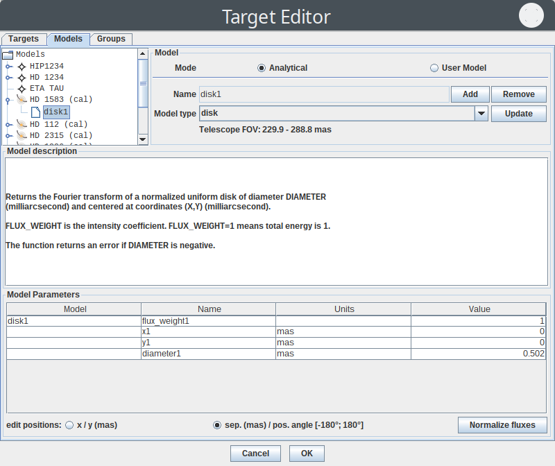
Target Editor

This window provides two tabbed panes to edit models and targets :

Model Tabbed Pane

The model editor allows you to edit the object model for one or several targets using an common interface with JMMC LITpro software. This window is modal i.e. changes are only effective when you click on the OK button or you close this window.

In the tree view at the top left targets with their models are shown.

To add a new elementary model, you choose first its model type and then click add.

Of course, you can convert any elementary model to another type when you select a model in the tree view, choose the new model type and click on the Update Button. Please check then the parameter values and correct them as wanted.

Supported elementary analytical models are :

• punct -ual object
• disk with elongated and flattened variants
• circle i.e. unresolved ring
• ring with elongated and flattened variants
• gaussian distribution with elongated and flattened variants
• limb darkened disk

Note

The supported model list is subject to change and evolve in the future.

The Model description area gives you a description of the elementary model and its parameters.

The Model Parameters table let you edit each parameter of analytical models.

When several models are defined for a target, the first model is always centered (x = y = 0). Positions of other models can be edited using polar coordinates rho and theta (-180;180) according to edit positions choice.

The Normalize fluxes button corrects the values of the flux_weight parameter to have a total flux equal to 1.

Target Tabbed Pane

TODO

Preferences

This window let you define several settings that are stored on your machine and will be loaded at application start up.

Use the Default settings to reset your preferences to default values and Save to make you changes persistent; otherwise, your settings will be used until you close ASPRO 2.

Interoperability

ASPRO 2 uses the SAMP VO protocol (see IVOA Samp for more information) to provide interoperability with other JMMC applications and in the future with other VO applications (VO stands for virtual observatory).

ASPRO 2 / SearchCal

How to find calibrators using SearchCal from ASPRO 2 ?

Here is a step by step tutorial :

1. Start SearchCal application (if needed)

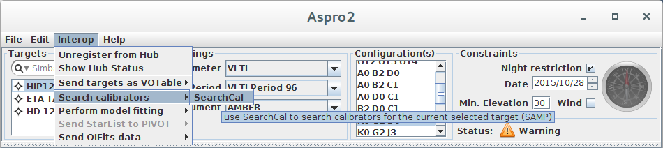
1. In ASPRO 2, use the Search calibrators action in the Interop Menu to let ASPRO 2 tell SearchCal to search calibrators for the selected target in the main panel :

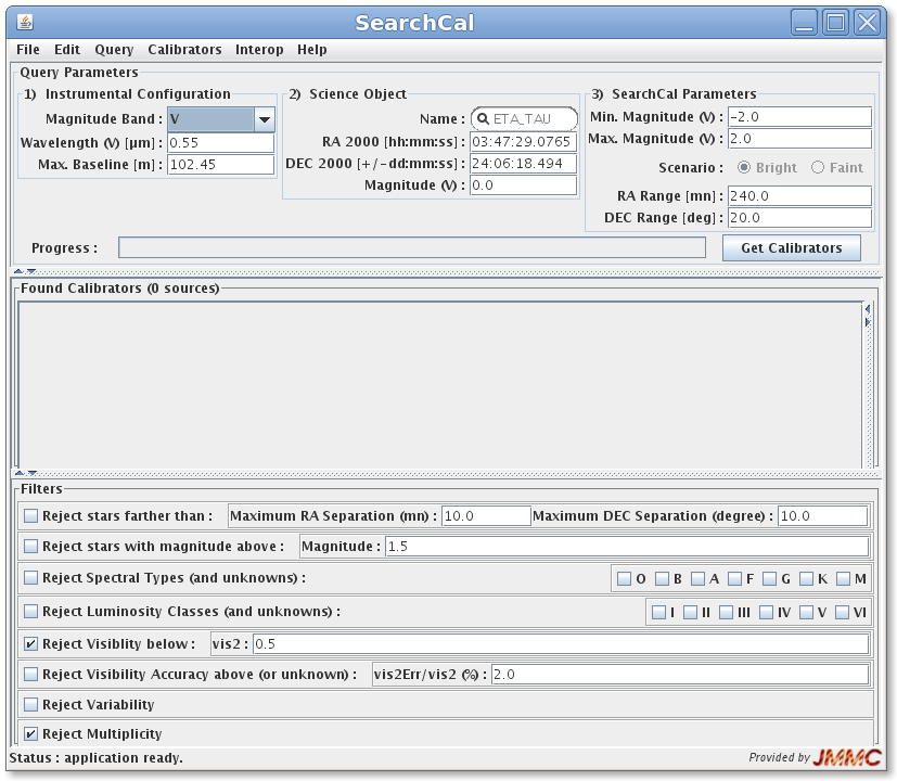
1. SearchCal executes the ASPRO 2 query (please wait ...)

1. SearchCal gets results from the JMMC server

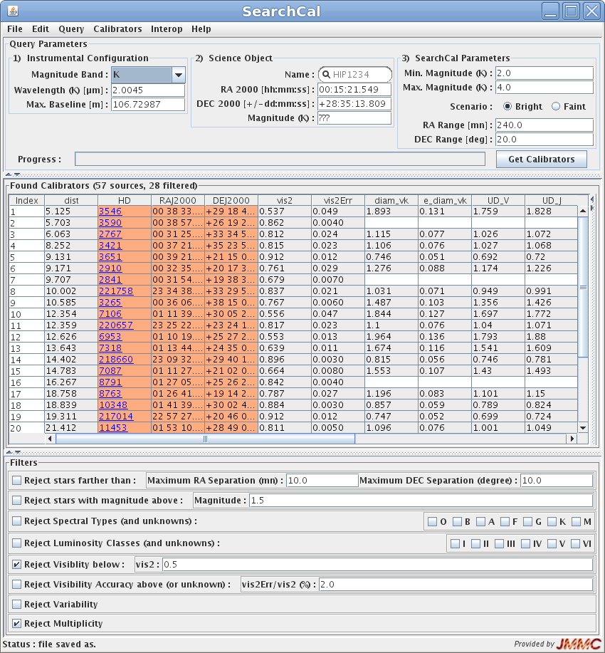
1. Select the calibrators you want to use and use the Send calibrators to action in the Interop Menu to let SearchCal send calibrators back

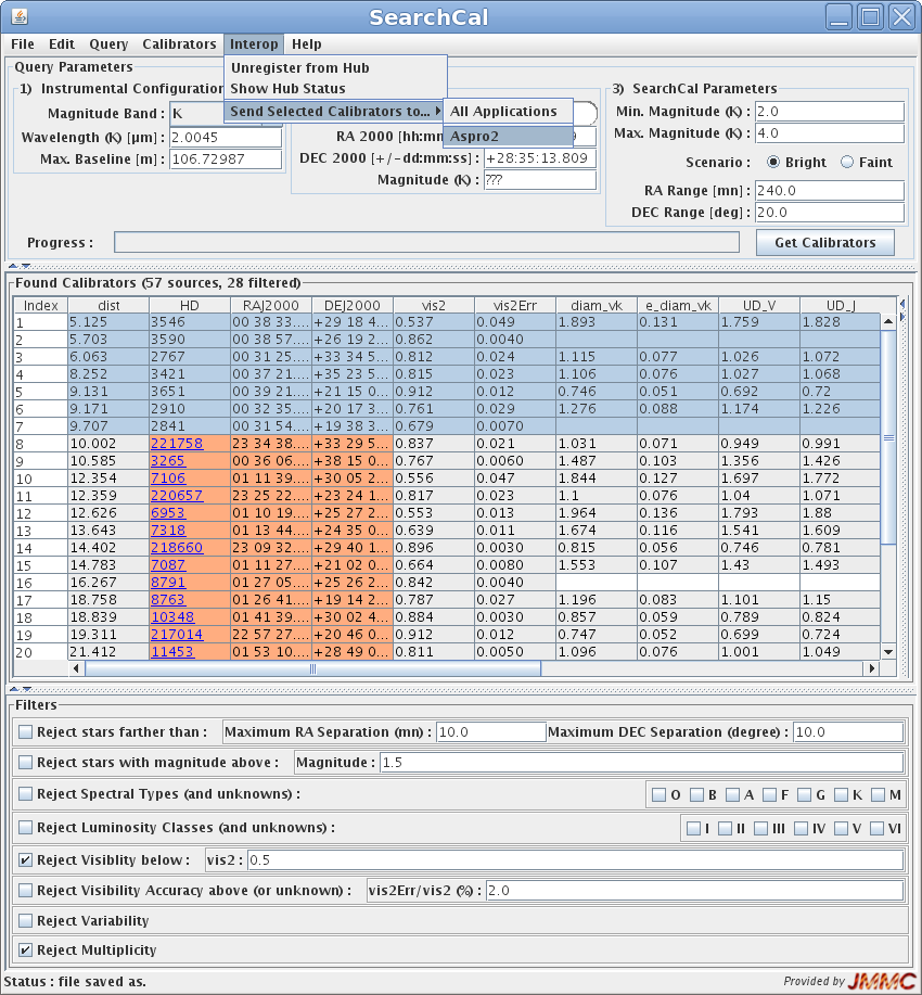
1. ASPRO 2 processes the SearchCal calibrators and displays a summary

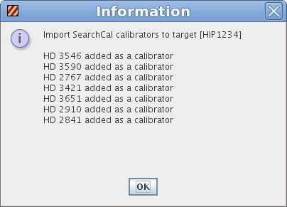
1. That's all : ASPRO 2 has now updated the target list with the SearchCal calibrators (associations) and plots are updated :

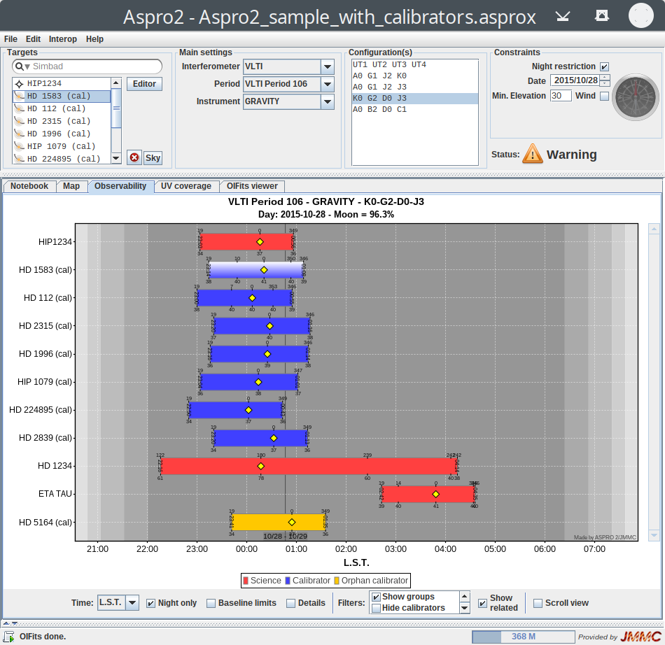
• Observability plot with calibrators below science target

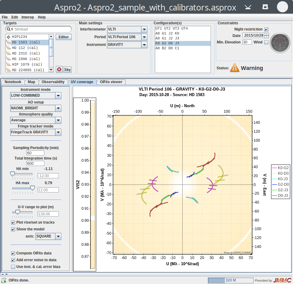
• UV Coverage plot for a calibrator

• Target editor with calibrators
  • Target tabbed pane :

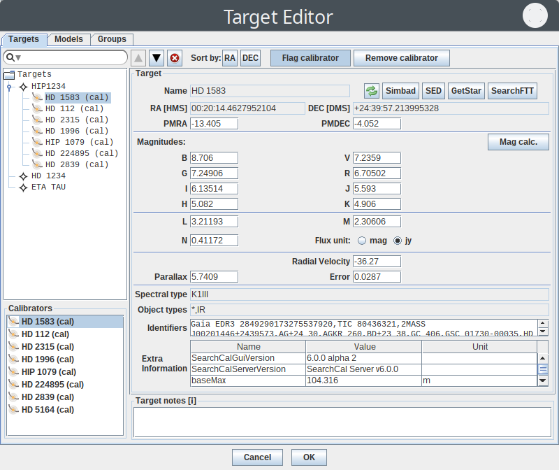
• • Model tabbed pane for a calibrator :

TODO

ASPRO 2 / LITpro

TODO

Sample files

Here are the "Guided Tour" Observation files that can be loaded in ASPRO 2 for demonstration purposes.

• Aspro2_sample.asprox: Sample observation file
• Aspro2_sample_with_calibrators.asprox: Sample observation file with SearchCal calibrators

Support and requests of changes

Please do not hesitate to contact the user support team for any bug report or change request.